Calculating Yaw of Repose and Spin Drift (short form)
-A novel and practical approach for computing the Spin Drift perturbation-
James A. Boatright & Gustavo F. Ruiz
- Introduction
- Framework of the Analytical Solution
- PRODAS Simulated Flight Data
- Estimating the Yaw of Repose
- Analytic Calculation of the Spin Drift at the Target
- Estimating the Spin Drift Scale Factor – ScF
- Calculating the Spin Drift at the Target
- Example Calculations of Spin Drift
- Closing summary
Introduction
The Yaw of Repose angle
β[SUB]R[/SUB] is a very small, but gradually increasing, horizontally rightward, aircraft-type yaw-attitude bias or “side-slip” angle of the
coning axis of a right-hand spinning bullet. The Yaw of Repose reverses sign and angles leftward for a left-hand spinning bullet.
We discuss only right-hand spinning bullets here for clarity. It can be shown that for right-hand twist, the yaw of repose lies to the right of the trajectory. Thus the bullet cones around with an average attitude offset to the right, leading to increasing side drift to the right.
For spin-stabilized bullets, this attitude angle creates the well known horizontally rightward Spin Drift displacements on long-range targets. The small horizontally rightward Yaw of Repose angle causes a small rightward aerodynamic lift force which, in turn, causes a slowly increasing horizontal velocity of the bullet.
It is important to realize that this effect occurs independently of the presence of surface wind of any force or from any direction. Bear in mind that the Yaw of Repose represents the horizontal yaw attitude of the bullet’s
coning axis or the average yaw of the coning bullet.
The acceleration of gravity acting upon the flat-fired bullet in free flight is the original cause of this small yaw-attitude bias angle. The downward curving of the trajectory due to gravity causes the airstream passing over the bullet to approach from below the nose of that bullet.
This wind shift during each coning cycle causes an increased aerodynamic angle of attack which peaks when the center of gravity (CG) of the bullet is at the Bottom Dead Center (BDC) position in each coning cycle where its nose is oriented maximally upward.
FIGURE: Extreme TDC and BDC Positions of the Coning Bullet
Since the coning angle
α always exceeds this small change in the approaching airstream direction during each coning cycle, the aerodynamic angle of attack for a bullet at Top Dead Center (TDC) when the bullet’s nose is pointing maximally downward is at a minimum for that coning cycle.
These modulations of aerodynamic angle of attack during each coning cycle produce small differential rightward-acting increments in the aerodynamic overturning moment experienced by the bullet centered upon the BDC and TDC positions of the bullet during each coning cycle.
In physics these are termed “torque impulses,” and each one pushes the angular momentum vector of the right-hand spinning bullet horizontally rightward without affecting its spin-rate. Torqueing the angular momentum vector of the spinning bullet rightward is tantamount to turning the nose of the flying bullet rightward.
Both the overturning moment vector
M and its differential torque impulse vector
ΔM point rightward for the bullet at its BDC location. While the vector
M itself points leftward as seen from behind when the bullet is located at TDC in its coning cycle, the
reduced angle of attack at that position produces a
negative differential vector
ΔM which is
positive rightward at TDC as well.
The 175.16-grain 30-caliber US Army M118LR bullet used as an example here is experiencing its 88[SUP]th[/SUP] half-coning cycle when it reaches the target distance of 1,000 yards. The reinforcing cumulative effect of this chain of rightward torque impulses occurring twice per coning cycle (or once each half cycle) is the mechanism by which gravity causes the slowly increasing rightward Yaw of Repose attitude bias of the flying bullet.
Framework of the Analytical Solution
The horizontal spin-drift
SD which we observe in long-range shooting is due to a horizontally acting aerodynamic
lift force attributable to the small, but steadily increasing, Yaw of Repose attitude angle
β[SUB]R[/SUB] of the coning rifle bullet.
We will use the principles of linear aeroballistics in formulating the Yaw of Repose and its resulting Spin-Drift.
Detailed analyses of PRODAS 6-DoF simulation runs show that in flat firing the magnitude of the spin-drift
SD in any given simulated firing is, beyond the first 150 yards or so,
very nearly equal to some invariant Scale Factor
ScF of about
1.2 to
2.4 percent, more or less, times the bullet’s
drop from the projected bore axis:
SD(t) = ScF*DROP(t) (1)
In other words, the horizontal spin-drift trajectory looks just like a small fraction
ScF of the vertical trajectory rotated 90 degrees about the extended axis of the bore with both curvatures ultimately caused by the same gravitational effect.
We must formulate the Scale Factor
ScF so that it can be accurately evaluated for any given bullet type and firing conditions.
After calculating the Scale Factor
ScF, we need only an accurate determination of the bullet’s
drop from the bore axis at the target distance to calculate an accurate Spin-Drift at the target.
Existing 3-DoF trajectory programs specialize in the accurate calculation of this bullet drop at the target distance in any firing conditions.
PRODAS Simulated Flight Data
In this paper we will use as our example bullet the 30-caliber 175-grain “M118LR” bullet as loaded in the US Army’s M118LR Special Ball (7.62x51 mm NATO) long-range sniper and match ammunition. We do this because we have several PRODAS 6-DoF simulation runs on hand (from 2011) for this 7.62 mm NATO ammunition, reporting the linear ballistic results (including Spin-Drift) for each millisecond of its
1.6923-second total simulated flight time to
1000 yards.
The bullet weight actually used in these PRODAS runs is
175.16 grains. The simulated firing conditions are 1) flat firing, 2) standard sea-level ICAO atmosphere, 3) no wind, 4) no Coliolis effect calculated, 5) muzzle velocity of
2600.07 feet per second, and 6) barrel twist is right-handed at
11.5 inches per turn.
The “no-wind” and “no-Coliolis” conditions assure that the rightward spin-drift
SD is the only secular horizontal “bullet drift” being computed by PRODAS. However, the PRODAS reported drift data necessarily includes the oscillating horizontal component of the bullet’s helical coning motion about its mean trajectory throughout its simulated flight.
We also have PRODAS runs available for this same bullet fired through constant left and right 10 MPH crosswinds as well as left-hand twist runs in each of the three constant wind conditions.
Estimating the Yaw of Repose
Based upon the above gravitational explanation, we have developed an integral expression for the Yaw of Repose angle
β[SUB]R[/SUB](t) at any flight time
t which well matches the available PRODAS data for this example M118LR bullet:
β[SUB]R[/SUB](t) = (2π*g/t)∫[ω[SUB]2[/SUB](t)*V(t)][SUP]-1[/SUP] dt (2)
where
g = 32.174 feet/second[SUP]2[/SUP] is the acceleration of gravity,
ω[SUB]2[/SUB](t) is the instantaneous coning (or gyroscopic precession) rate of the bullet in radians per second, and
V(t) is the instantaneous forward velocity of the bullet in feet per second.
In the absence of having 6-DoF simulation data available, we could approximate the Yaw of Repose angle
β[SUB]R[/SUB](t) by assigning (closed form) integrable continuous functions of time
t to represent the variables
ω[SUB]2[/SUB](t) and
V(t) so that we could then approximate this
summing operation by performing the definite integration.
If we calculate the values of
ω[SUB]2[/SUB](t) and
V(t) at
t = 0 and at a much later flight time
t = T, and we assume for approximation purposes that each function decays exponentially with time
t, then the definite integral for
β[SUB]R[/SUB](t) can be expressed as:
β[SUB]R[/SUB](t) = {2π*g/[ω[SUB]2[/SUB](0)*V(0)*T]} ∫exp[-(kω + k[SUB]V[/SUB])*t/T] dt (3)
with
kω = ln[(ω[SUB]2[/SUB](T)/ω[SUB]2[/SUB](0)]
ω[SUB]2[/SUB](t) = ω[SUB]2[/SUB](0)*exp[kω*t/T] (4)
k[SUB]V[/SUB] = ln[V(T)/V(0)]
V(t) = V(0)*exp[k[SUB]V[/SUB]*t/T] (5)
Here we are using
t/T as a dimensionless canonical variable in the exponential decay expressions and as a dummy variable in the (summing) integration.
After the definite integration from
t = 0 to
t =T, the expression for
β[SUB]R[/SUB](t) is:
β[SUB]R[/SUB](t) = {-2π*g/[ω[SUB]2[/SUB](0)*V(0)*(kω + k[SUB]V[/SUB])]}*{exp[-(kω + k[SUB]V[/SUB])*t/T] - 1} (6)
Our “no wind” PRODAS runs for this M118LR bullet show that
V(t) slows from an initial velocity of
2600.07 feet per second to
1340 FPS (Mach 1.20) at
888.5 yards downrange with a time-of-flight (
T) of
1.430 seconds, and the coning rate
ω[SUB]2[/SUB](t) of the bullet slows from
2π*45.57 radians per second to
2π*17.00 radians per second over this same interval of
T seconds.
The Yaw of Repose
β[SUB]R[/SUB](T) at
T = 1.430 seconds, and at
888.5 yards downrange, would then be calculated as:
kω = ln[(ω[SUB]2[/SUB](T)/ω[SUB]2[/SUB](0)] = -0.98604
k[SUB]V[/SUB] = ln[V(T)/V(0)] = -0.66328
β[SUB]R[/SUB](1.430 sec) = [1.6464x10[SUP]-4[/SUP]]*[4.20344] = 0.69206 mrad = 0.039652 degrees (7)
While PRODAS does not directly report
β[SUB]R[/SUB], this small
0.040-degree angle is not unreasonable for this M118LR bullet at
888.5 yards downrange, and it matches the horizontal deviation in the trajectory simulation quite well.
We will use this closed-form algorithm (
Eq. 6) for estimating the Yaw of Repose angle
β[SUB]R[/SUB](t) without relying upon 6-DoF simulation data in formulating the spin-drift
SD(t) of any rifle bullet at long ranges.
Analytic Calculation of the Spin Drift at the Target
If we formulate a reliable estimation of the Scale Factor
ScF for any given bullet in any given firing conditions, this Scale Factor
ScF can then be used together with a reliably calculated value of that bullet’s
DROP from the bore axis at the target to calculate analytically the spin-drift
SD(t) at the target for any given rifle bullet in any firing conditions according to
Eq. 1:
SD(t) = ScF*DROP(t)
We know from examination of available “constant crosswind” PRODAS 6-DoF simulations that the Scale Factor
ScF needs to be
0.0219685 for the “constant no-wind” runs, and
0.0222219 (or 1.154 percent larger) for the “constant 10 MPH crosswind” runs for this example M118LR bullet fired in these simulated conditions to
1,000 yards.
The constant “no-wind” case represents the
minimum possible SD(t) values for this bullet fired at this muzzle velocity and spin-rate in this atmosphere and flying with the
minimum possible coning motion throughout its flight.
Most
dynamically stable rifle bullets fired outdoors at long ranges will likely suffer only the minimal
1.154 percent increased “constant 10 MPH crosswind” type of spin-drift
SD(t) at long ranges.
However, a
dynamically unstable rifle bullet, such as the infamous mid-range 30-caliber 168-grain Sierra International, might experience about
5 percent greater spin-drift (
SD) when fired to long ranges (up to 800 meters) through
any non-zero crosswinds. The PRODAS data show that the M118LR bullet is considered to be dynamically stable in supersonic flight.
Estimating the Spin Drift Scale Factor - ScF
We formulate an estimator for an
ScF value of the “constant 10 MPH crosswind” type of coning motion for our example bullet which can be duplicated for any other
dynamically stable bullet in any likely firing conditions.
In flat firing, we can formulate this Scale Factor
ScF in terms of the
ratio of 1) the horizontal aerodynamic lift-force acting on the flying bullet due to its Yaw of Repose
β[SUB]R[/SUB] as that bullet nears its long-range target to 2) the vertically downward-acting weight of that bullet. In this manner, we can formulate
ScF for any given bullet and likely wind conditions as:
ScF = 1.01154*0.383703*[q(t)*S]*SIN[β[SUB]R[/SUB](t)]*CL[SUB]β[/SUB](t)/Wt
ScF = 0.388132*[q(t)*S]*β[SUB]R[/SUB](t)*CL[SUB]β[/SUB](t)/Wt (8)
with
Wt = 175.16/7000 representing the weight of this bullet given in pounds-force
lbf.
The initial constants (
0.383703 and
0.388132) have been empirically determined from several PRODAS runs and should be the same for any
dynamically stable rifle bullet in any firing conditions likely to be encountered in long-range rifle shooting.
These PRODAS simulations, together with the classic formulation for the yaw of repose angle
β[SUB]R[/SUB](t), indicate that the Scale Factor
ScF might need to be increased by about
5 percent for
marginally dynamically unstable bullets which will fly with significant coning angles throughout their flight when fired through
any non-zero crosswinds.
Each of these functions of time
t should be evaluated at the time
T when the bullet has slowed to an airspeed of
1340 feet per second, or approximately
Mach 1.20, depending upon ambient conditions.
This flight time
T and the flight distance at which it occurs are completely independent of the actual range to the target. The time
T can be determined by using a 3-DoF point-mass trajectory calculator.
Any good long-range rifle bullet should remain safely above the turbulent transonic region at this
1340 fps airspeed in almost all atmospheric conditions.
The more “aerodynamic” of our lowest-drag long-range rifle bullet designs do not encounter transonic buffeting until they slow to about
Mach 1.10 airspeed. The needed coefficient of lift
CL[SUB]β[/SUB] is particularly difficult to estimate for any bullet at transonic airspeeds.
Most experienced long-range riflemen select their shooting equipment so that whenever possible their bullets impact the target at airspeeds above
Mach 1.2
For similar best-accuracy reasons, we base our calculation of
ScF upon bullet data at
1340 fps airspeed regardless of the actual range to the intended target.
We calculate the potential drag-force
q(T)*S using the calculated density
ρ of the ambient atmosphere in
slugs per cubic foot, and the airspeed
V(T) = 1340 feet per second:
q(T)*S = [(ρ/2)*(1340 fps)[SUP]2[/SUP] ]*[(π/4)*d[SUP]2[/SUP] ] (9)
This potential drag-force value should be about
1.1 lbf for a
30-caliber bullet at this airspeed depending on air density. The potential drag-force at
1340 fps varies most strongly with the square of the caliber
d(in feet) of the bullet. The actual drag force
F[SUB]D[/SUB] experienced by the bullet flying at any given airspeed is this potential drag force multiplied by that bullet’s coefficient of drag
CD for the Mach-speed corresponding to that airspeed.
While the drag coefficient
CD of a rifle bullet
increases as its airspeed slows in supersonic flight, the actual drag force
F[SUB]D[/SUB] which it experiences continually
decreases during its supersonic flight. This net reduction is caused by the dynamic pressure
q decreasing even more rapidly with
V[SUP]2[/SUP] as the bullet slows.
The analytic estimate of
β[SUB]R[/SUB](T) is calculated per
Eq. 6 above with
t = T and
V(T) = 1340 fps. With these simplifications
Eq. 6 becomes:
β[SUB]R[/SUB](T) = -g*{exp[-(kω + k[SUB]V[/SUB])] - 1}/[f[SUB]2[/SUB](0)*V(0)*(kω + k[SUB]V[/SUB])] (10)
If we know the
initial gyroscopic stability
Sg of the bullet, we can calculate the initial Stability Ratio
R of its epicyclic rates
f[SUB]1[/SUB]/f[SUB]2[/SUB] from:
R = 2*{Sg + SQRT[Sg*(Sg – 1)]} – 1 (11)
The
initial coning rate
f[SUB]2[/SUB](0) in hertz can then be found from Tri-Cyclic Theory as:
f[SUB]2[/SUB](0) = V(0)/[Tw*(Iy/Ix)*(R + 1)] (12)
where
Tw = Absolute value of the Twist Rate of barrel in feet per turn.
Iy/Ix = Ratio of transverse to axial second moments of inertia for this bullet. [An algorithm for estimating
Iy/Ix with reasonable accuracy is explained in the detailed version of this paper. It should also be used for this
Iy/Ix calculation in the earlier CWAJ paper.]
Substituting back into
Eq. 10, we have:
β[SUB]R[/SUB](T) = -g*Tw*(Iy/Ix)*(R + 1)*{exp[-(kω + k[SUB]V[/SUB])] - 1}/[V[SUP]2[/SUP](0)*(kω + k[SUB]V[/SUB])] (13)
where
V(0) = Launch velocity of this particular bullet in feet per second. [
V(0) is assumed to exceed
Mach 2.0]
kω = -0.98604, as before for any long-range bullet, and
k[SUB]V[/SUB] = ln[1340/V(0)].
This value
β[SUB]R[/SUB](T) in radians is the estimated Yaw of Repose angle for this bullet when it has slowed to
1340 fps.
The coefficient of lift value
CL[SUB]β[/SUB](T) is evaluated based on an estimate of the initial
CL[SUB]β[/SUB](0) for the Mach-speed of the bullet at launch (here
Mach 2.3289) from Robert L. McCoy’s INTLIFT program for the nose-length effect, but using our own boat-tail effect lift reduction for these long-range bullets.
We multiply McCoy’s nose-length estimated
CL by the square root of
0.2720/BC7 for each bullet, reasoning that about half of any differing drag for bullets having higher or lower ballistic coefficients
BC7 (Ballistic Coefficient relative to the G7 Reference Projectile) than our example M118LR bullet is due to having a more or less effective boat-tail design.
If a more reliable
BC1 value (BC relative to the G1 Reference Projectile) is available for your rifle bullet, use the square root of
0.5460/BC1 for this
CL adjustment for bullet drag.
Very slightly scaling McCoy’s published lift curve for the well-studied 30-caliber 168-grain Sierra International bullet to this lift coefficient
2.720 at this
Mach 2.3289 airspeed yields a coefficient of lift
CL[SUB]β[/SUB](T) of
1.877 at
Mach 1.20 in this standard sea-level ICAO atmosphere.
The bullet’s zero-yaw coefficient of drag
CD[SUB]0[/SUB]function determines its time-rate of decay in Mach-speed. The supersonic lift-to-drag ratio
F[SUB]L[/SUB]/F[SUB]D[/SUB] for any given angle-of-attack tends to be an invariant aerodynamic characteristic of each basic bullet shape.
Since the coefficients of lift and drag are highly correlated at any given Mach-speed over the rather similarly shaped population of long-range rifle bullets, the same exponential time-decay coefficient:
k[SUB]L[/SUB] = ln[CL[SUB]β[/SUB](T)/ CL[SUB]β[/SUB](0)] = -0.3711 (14)
can be used in calculating the coefficient of lift
CL[SUB]β[/SUB](T) for any long-range rifle bullets of interest here.
We propagate this
initial coefficient of lift
CL[SUB]β[/SUB](0) estimate forward to its value at time
T as:
CL[SUB]β[/SUB](T) = CL[SUB]β[/SUB](0)*EXP[-0.3711*(V(0)/2600 fps)[SUP]2[/SUP] *(1.430 sec/T)] (15)
The coefficient of lift
CL[SUB]β[/SUB](T) for any very-low-drag (VLD) or ultra-low-drag (ULD) long-range rifle bullet should be smaller than
1.90 at this airspeed of
1340 fps. Bullets designed for lower aerodynamic drag by incorporating an effective boat-tail design will also produce less aerodynamic lift. Conversely, you cannot produce more lift without also increasing drag in aerodynamics.
The exponential propagation function [
Eq. 47] estimates a larger fraction of the initial coefficient of lift
CL[SUB]β[/SUB](0) remaining at
1340 fps airspeed when the time-of-flight
T to that airspeed is increased due to firing a higher-drag bullet, but the initial velocity correction factor [
V(0)/2600 fps][SUP]2[/SUP] prevents this increase when time-of-flight
T to
1340 fps increases simply due to firing that same bullet at a higher muzzle velocity
V(0). That is, if the
same bullet is fired at different muzzle velocities, its estimated coefficient of lift
CL[SUB]β[/SUB](T) at
1340 fps airspeed should remain the same.
The muzzle velocity
V(0) is assumed always to exceed
Mach 2. This coefficient of lift propagation yields the expected
CL[SUB]β[/SUB](T) = 1.8769 at
1340 fps for the M118LR bullet, and varies by less than
1 percent over any reasonable launch speeds
V(0) for this one bullet type.
The scale factor
ScF is now calculated from
Eq. 8 using the values of the time-functions at time
T as calculated in
Eq. 9,
Eq. 13, and
Eq. 15 above:
ScF = 0.388132*[q(T)*S]*β[SUB]R[/SUB](T)*CL[SUB]β[/SUB](T)/Wt (16)
If we might be slightly misestimating the Yaw of Repose angle
β[SUB]R[/SUB](T) or coefficient of lift
CL[SUB]β[/SUB](T) used here in any systematic ways for these minimal-coning-motion “constant wind” 6-DoF flight simulations, the empirically-determined initial constant factor
0.388132, from that same PRODAS data, tends to absorb any net difference.
Calculating the Spin Drift at the Target
The spin-drift
SD(tof) at the
target distance is then calculated from
Eq. 1 above using the invariant Scale Factor
ScF, as calculated in
Eq. 16 above, and the total
DROP from the axis of the bore for the time-of-flight (
tof) to the target:
SD(tof) = ScF*DROP(tof) (17)
The Spin-Drift
SD at the target is calculated here in
Eq. 17 in the same
distance or
angular units in which the bullet’s
DROP from the bore axis is given. The proper sign depends upon coordinate system conventions and the sense of the bullet’s spin.
The bullet
DROP and time-of-flight (
tof) to the target are accurately calculated in many existing 3-DoF point-mass trajectory propagators. After all, the accurate calculation of bullet
DROP at the target distance is the basic figure of merit for these software aids.
The time-of-flight (
tof) to the target is used in the Litz
SD estimator and is nice to know even if we do not actually need it in these calculations.
If your particular trajectory propagation program does not directly output “drop from bore axis” data, you can usually “fake” it into doing so by setting your scope height equal zero, setting the angle-of-fire accurately equal to that of the anticipated shot, setting the rifle’s “zero range” equal to some minimum distance (ideally zero, or 5 or 10 yards if made necessary by input limit constraints), and specifying that the trajectory calculations go out to the target’s known range.
In other words, we want to calculate the
DROP from the bore axis at the target distance as if we were “bore-sighted” on that long-range target.
The smoothed spin-drift reported by PRODAS at 1000 yards for “constant zero-wind” simulations with this M118LR bullet fired in these conditions is
9.5407 inches. The spin-drift
SD estimated via this algorithm for 1000 yards (without the factor of
1.01154 increase in
ScF) is
9.5635 inches.
Comparing the two results millisecond-by-millisecond throughout the flight of
1692.3 milliseconds, yields a mean difference of
0.0043 inches with a population standard deviation of
0.0207 inches.
This level of agreement between our analytical estimator for spin-drift for each millisecond and the PRODAS numerical simulation results is rather astonishing. The rounding error for drop and drift data in the PRODAS report format is
0.180 inches at 1000 yards, and we are not even estimating the horizontal component of the bullet’s small coning motion which is included in the PRODAS drift data.
The agreement of this spin-drift
SD estimator with PRODAS “constant 10 MPH crosswind” runs is almost as good when the Scale Factor
ScF includes the
1.154 percent increase as formulated above.
This
1.154-percent-augmented version of
ScF in
Eq. 8 should be calculated for firing any
dynamically stable rifle bullets outdoors.
Example Calculations of Spin Drift
The parameters needed to calculate Yaw of Repose
β[SUB]R[/SUB] and spin-drift
SD are calculated for the five example bullets in the spreadsheet shown below. A 3-DoF trajectory program was used to compute the time-of-flight (
tof) and flight distance to an airspeed of
1340 FPS and
tof to a 1000-yard target for the 168-grain SMK bullet, the new 173-grain ULD bullet, and the two Berger 30-caliber bullets tested by Bryan Litz. PRODAS trajectory data was used for the M118LR bullet.
The initial gyroscopic stability factor
Sg was taken from McCoy for the old 168-grain Sierra International bullet (and applied to the 168-grain SMK), and
Sg is calculated using McCoy’s McGYRO program for the new 173-grain ULD bullet.
PRODAS reports the
Sg-value for each millisecond of the flight of the M118LR bullet, but we just used their initial value. Bryan Litz gives the initial
Sg values for the two Berger bullets used in his drift firings.
The ULD bullet is a dual-diameter design with the base of the ogive measuring
0.3002 inches in diameter (
1.0-calibers for this bullet design). It has a rear driving-band measuring
0.3082 inches in diameter (
1.02665 calibers).
The midpoint (CG) of the rear driving-band is located
1.6 calibers behind the base of its 3-caliber secant ogive, and the effective width of this driving band is
0.6 calibers.
Our calculated Yaw of Repose angles
β[SUB]R[/SUB] for the first three example bullets when each has slowed to an airspeed of
1340 FPS shows an interesting progression. The estimated Yaw of Repose angles
β[SUB]R[/SUB] of the three trajectories at the
1340 FPS airspeed points are
0.471231 milliradians for the obsolete 168-grain International bullet at
816 yards downrange, and
0.693417 milliradians at
888.5 yards downrange for the M118LR bullet, but just
0.434382 milliradians for the new 173-grain monolithic brass ULD bullet, and this occurs way beyond the 1000-yard target at
1457 yards downrange.
The assumed
3200 fps muzzle velocity of this ULD bullet is based on firing it from a 300 Remington UltraMag cartridge. Each of the other example 30-caliber bullets is assumed to be fired from a much less powerful 7.62 mm NATO or 308 Winchester cartridge.
For comparison purposes the spin-drift
SD at
1000 yards is calculated in inches for each of our five example bullets using the
SD estimator published by Bryan Litz:
SD(inches) = 1.25*(Sg + 1.2)*(tof)[SUP]1.83[/SUP] (18)
Our estimates of
SD at 1000 yards are
smaller than Bryan’s estimates for each of our five example bullets.
Our estimate of
7.0152 inches of spin-drift
SD at 1000 yards for the old 168-grain Sierra International bullet from a 12-inch twist barrel is approximately
2.135 inches less than the
9.15 inches shown graphically by McCoy in
Figure 9.8 of his MEB, and is
3.005 inches less than the
10.020 inches calculated by the Litz estimator for this bullet.
We expected our estimate to be at least
5 percent (or
0.458 inches) too small for this
dynamically unstable bullet. We cannot readily explain the remainder of this difference other than point to the unusually high coning rate
ω[SUB]2[/SUB](t) of this bullet throughout its flight due to its low
Iy/Ix ratio.
Our estimate of spin-drift
SD at 1000 yards for the M118LR bullet
9.7037 inches matches the
SD computed by PRODAS (
9.5407 inches) quite closely (error:
+0.163 inches, or
+1.708 percent).
We expected this value to be
1.154 percent too large because this PRODAS run is for the unrealistic “no wind anywhere” case causing absolute minimum coning motion of this bullet. Thus, the unexplained difference between our
SD estimate and that computed in PRODAS is
0.554 percent. The Litz-estimated
SD of
10.2791 inches for this M118LR bullet at 1000 yards exceeds the PRODAS value by
0.7156 inches, or
+7.483 percent.
Our estimate of
3.1214 inches of spin-drift
SD at 1000 yards for the radical new 173-grain monolithic brass ULD bullet design, versus the value of
5.1696 inches calculated by the Litz estimator for this bullet, indicates the need for our more elaborate
SD calculation in predicting the long-range flights of current and future ultra-low-lift rifle bullets, even when fired from faster twist-rate barrels.
The Litz spin-drift estimator is closer than our estimator to reported spin-drift values for the old 168-grain Sierra International bullet [McCoy] and for the Berger 175-grain OTM Tactical bullet [from Bryan’s own drift firings].
Our estimator seems closer for the remaining three bullets, especially for the two very-low-drag (and correspondingly very-low-lift) bullets—the brass 173-grain ULD bullet and the Berger 185-grain Long Range Boat-Tail (LR-BT) bullet.
Of course, our predictive agreement with the PRODAS calculations for the M118LR bullet is best of all. We suspect that if 6-DoF simulations could be run for the other four bullets, our estimator would match those results more closely.
We also suspect that Bryan’s drift firing results might not match linear 6-DoF aerodynamic flight simulation results particularly well if they could be computed.
The aerodynamic responses of real rifle bullets are non-linear enough to affect the calculation of these small second-order effects. Real bullets are also subject to other types of aerodynamic jump phenomena in real firings—some of which might be at least partially systematic.
| Spin-Drift Example Calculations: | | | | Temp (Degrees-F) | 37.00 |
| | Std ICAO Atmosphere: | | | Rel. Humidity | 70.00 |
| Rho (Lbm/Cu. Ft.) | 0.0764742 | 0.0764742 | 0.0764742 | Stat Pressure (InHg) | 28.9500 |
| Rho (Slugs/Cu.Ft.) | 0.002376894 | 0.0023768 | 0.002376 | 0.002397459 | 0.00239745 |
| Mach 1.00 = a (FPS) | 1116.45 | 1116.45 | 1116.45 | 1093.23 | 1093.23 |
| | | | | | |
| 30-Caliber Example Bullets: | 168-gr International | 175.16-gr M118LR | 173-gr ULD(SB) | 175-gr Berger Tactical | 185-gr Berger LR-BT |
| Bullet Length L (cal) | 3.9800 | 4.0260 | 5.4368 | 4.1169 | 4.3929 |
| Nose Length LN (cal) | 2.2600 | 2.3052 | 2.8368 | 2.3701 | 2.5747 |
| Diameter of Meplat DM (cal) | 0.2500 | 0.2175 | 0.1000 | 0.1948 | 0.2013 |
| Length of Boat-Tail LBT (cal) | 0.5100 | 0.5360 | 0.7012 | 0.6331 | 0.5844 |
| Diameter of Base DB (cal) | 0.7645 | 0.8280 | 0.8420 | 0.8409 | 0.8182 |
| Ratio of Ogive Generating Radii RT/R | 0.9000 | 1.0000 | 0.5000 | 0.9000 | 0.9500 |
| Calc. Tangent Ogive Radius RT (cal) | 6.9976 | 6.9866 | 9.1666 | 7.1779 | 8.4993 |
| Calc. Full Tangent Ogive Length LFT (cal) | 2.5976 | 2.5955 | 2.9861 | 2.6321 | 2.8722 |
| Calc. Full Conical Nose Length LFC (cal) | 3.0133 | 2.9459 | 3.1520 | 2.9435 | 3.2236 |
| Calc. Full Nose Length LFN (cal) | 2.6392 | 2.5955 | 3.0690 | 2.6632 | 2.8897 |
| | | | | | |
| V0=Launch velocity (FPS): | 2800.00 | 2600.07 | 3200.00 | 2660.00 | 2630.00 |
| Initial Mach-Speed | 2.5079 | 2.3289 | 2.8662 | 2.4332 | 2.4057 |
| Initial B-value | 2.3000 | 2.1032 | 2.6861 | 2.2182 | 2.1880 |
| Ballistic Coef (G1 Ref) | 0.4260 | 0.5460 | 0.6290 | 0.5060 | 0.5530 |
| Ballistic Coef (G7 Ref) | 0.2180 | 0.2720 | 0.3220 | 0.2580 | 0.2830 |
| INTLIFT CL(0) | 3.1015 | 2.7203 | 2.5551 | 2.8145 | 2.6189 |
| Time T to 1340 FPS (sec) | 1.2723 | 1.4300 | 2.1070 | 1.3972 | 1.5030 |
| Range at 1340 FPS Airspeed (yards) | 816.00 | 888.50 | 1457.00 | 881.5400 | 839.1000 |
| Est CL(T) at 1340 FPS: | 1.9120 | 1.8769 | 1.7447 | 1.8913 | 1.8248 |
| | | | | | |
| Twist Rate (inches/turn, RH) | 12.0000 | 11.5000 | 8.2500 | 10.0000 | 10.0000 |
| Initial Sg | 1.7400 | 1.9400 | 1.5940 | 2.2400 | 1.9100 |
| Initial Stability Ratio (R) | 4.7494 | 5.5808 | 4.1341 | 6.8132 | 5.4567 |
| Calculated (Iy/Ix) Ratio | 7.478685 | 9.067260 | 13.46233 | 9.7336 | 10.8488 |
| Initial Coning Rate f2 (hz) | 65.1188 | 45.4687 | 67.3429 | 41.9719 | 45.0549 |
| kv=LN(1340/V(0) | -0.736950 | -0.662869 | -0.870481 | -0.685657 | -0.674314 |
| komega+kv | -1.722990 | -1.648909 | -1.85652 | -1.671697 | -1.660354 |
| Beta-R at time T (mrad) | 0.471231 | 0.693417 | 0.434382 | 0.744921 | 0.696844 |
| | | | | | |
| Ref. Diam. (1.0 cal. in inches): | 0.3080 | 0.3080 | 0.3002 | 0.3080 | 0.3080 |
| Frontal Area S (square feet) | 0.000517403 | 0.0005174 | 0.000491 | 0.0005174 | 0.00051740 |
| Potential Drag Force at 1340 fps (lbf) | 1.1041 | 1.1041 | 1.0489 | 1.1041 | 1.1041 |
| | | | | | |
| Bullet Weight (grains) | 168.0 | 175.1600 | 173.0 | 175.0 | 185.0 |
| Bullet Weight (lbf) | 0.0240000 | 0.0250229 | 0.02471 | 0.02500 | 0.0264286 |
| Calculated Scale Factor ScF | 0.016088267 | 0.0222895 | 0.012484 | 0.0241500 | 0.02061980 |
| | | | | | |
| DROP from Bore Axis at 1000 yds (inches) | 436.0450 | 435.3450 | 250.0250 | 428.4970 | 414.8350 |
| Time of Flight (tof) to 1000 yds (seconds) | 1.7300 | 1.6923 | 1.2390 | 1.6870 | 1.6400 |
| Remaining Velocity at 1000 yds (FPS) | 1145.00 | 1213.99 | 1836.00 | 1197.00 | 1278.00 |
| DROP from Bore Axis at 100 yds (inches) | 2.5500 | 2.6750 | 2.1400 | 2.7950 | 2.8550 |
| Calc. 100-yard SD (inches) | 0.0410 | 0.0596 | 0.0267 | 0.0675 | 0.0589 |
| Calculated 1000-yd Spin-Drift (inches rightward) | 7.0152 | 9.7036 | 3.1214 | 10.3482 | 8.5538 |
| SD from McCoy Figure 9.8 | 9.1500 | | | | |
| SD from PRODAS runs | | 9.5407 | | | |
| SD (inches) from Drift Firings | | | | 11.4000 | 6.7000 |
| Litz Est. Spin-Drift (inches rightward) | 10.0203 | 10.2791 | 5.1696 | 11.1967 | 9.6125 |
| Litz Est. Spin-Drift Minus Our Calc. SD (inches) | 3.0051 | 0.5754 | 2.0482 | 0.8485 | 1.0586 |

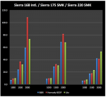
The Spin Drift is expressed in inches, while each bullet is compared with the three different estimators, and grouped at 1000, 1500 and 2000 yards, which are typical ranges for extended Long Range shooting.
The Litz estimator does fair work, given its simple inputs, but its reliability is dictated by the underlying aerodynamics characteristics of the bullet, which are not accounted for in this simple linear approach.
Consequently, as soon as the bullet does not exhibit certain properties that cannot be encompassed by
Sg alone, its predictive accuracy is decidedly affected. In general terms, the Litz model tends to over predict
SD in a significant way.
As can be appreciated, as the range increases, the difference among the estimators becomes larger. The practical side of this is that the correct method is of paramount importance when dealing with Extreme Long Range shooting.
Closing Summary
Taken together, the implications of
Eq. 8 and
Eq. 19 determine the bullet and rifle characteristics which affect the size of the horizontal spin-drift
SD(t) which will be seen in flat firing at a long-range target.
First, we see from
Eq. 8 that
SD(t) displacement is always proportional to the bullet’s
DROP(t) in distance units from the projected axis of the bore at firing. This implies that modern lighter-weight “flat shooting” bullets fired at higher muzzle velocities
V(0) and retaining more velocity farther downrange (higher ballistic coefficient, lower drag bullets) will produce much less spin-drift
SD(t) at any target distance compared to slower, higher-drag bullets. That is, here
SD(t) is roughly proportional to time-of-flight
t to the target distance.
Second, according to
Eq. 19, the size of the scale factor
ScF, and thence the size of the spin-drift
SD(t), varies directly with the “potential ballistic drag force”
q(t)*S = ρ*V[SUP]2[/SUP](t)*S/2 in pounds
. The ambient atmospheric density
ρ varies with shooting conditions. The rifle bullet’s retained velocity
V(t) depends upon its muzzle velocity
V(0), its mass
m, and the integrated drag function
CD[SUB]α[/SUB] of that bullet. The bullet’s cross-sectional area
S = π*d[SUP]2[/SUP]/4 varies with the square of the bullet’s caliber
d.
Third, the spin-drift
SD(t) of the bullet is proportional to its yaw-of-repose angle
β[SUB]R[/SUB](t) throughout its flight:
β[SUB]R[/SUB](t) = (2π*g/t)∫[ω[SUB]2[/SUB](t)*V(t)][SUP]-1[/SUP] dt
Both the coning rate
ω[SUB]2[/SUB](t) and the forward velocity
V(t) of the bullet always gradually decrease, continually increasing
β[SUB]R[/SUB](t) throughout the bullet’s flight. The coning rate
ω[SUB]2[/SUB](t) is determined by the bullet’s fixed inertial ratio
Iy/Ix and by the remaining spin-rate
ω(t) and slowly increasing gyroscopic stability
Sg of the flying bullet. The forward velocity
V(t) of the flying bullet depends on its launch velocity
V(0) and its coefficient of drag profile.
The yaw-of-repose attitude angle
β[SUB]R[/SUB](t) is
increased for bullets having larger numerical
Iy/Ix ratios and higher initial stability
Sg, but
β[SUB]R[/SUB](t) is
decreased by using faster twist-rate barrels and higher muzzle velocities
V(0) to achieve that higher gyroscopic stability
Sg.
Fourth, the spin-drift
SD(t) is directly proportional to the small-yaw coefficient of lift
CL[SUB]β[/SUB](t) of the bullet. Very-low-drag (VLD) and ultra-low-drag (ULD) bullet designs usually have correspondingly reduced coefficient-of-lift functions at all supersonic airspeeds.
Fifth, and lastly, the spin-drift
SD(t) of the bullet is inversely proportional to the weight
Wt (or mass
m) of that bullet.
All else being equal, bullets made with lower average material densities, such as turned brass bullets, will weigh less and will suffer greater spin-drift.
These five
SD effects combine multiplicatively in this analysis. Some bullet and rifle design parameters recur in several of these different
SD effects, and not always working in the same direction.
As modern long-range rifles and their bullets seem to be evolving toward lighter-weight, smaller-caliber, lower-drag bullets fired at higher muzzle velocities, these related incremental variations in design parameters combine algebraically to
reduce the spin-drift SD occurring on long-range targets.
Disclaimers & Notices
The findings in this report are not to be construed as an official position by any individual or organization, unless so designated by other authorized documents.
Citation of manufacturer’s or trade names does not constitute an official endorsement or approval of the use thereof.
Free and public distribution of this document is unrestricted and encouraged.